Default models

Examples of common models are shown below.

from comod import models

from IPython.display import display, Math

def show_graph(model):
    return model.plot_tikz(
        layout={s: (i, 0) for i, s in enumerate(model.states + [model.nihil_state])},
        edge_curved=0.3
    )

def show_latex(model):
    display(Math(model.to_latex()))

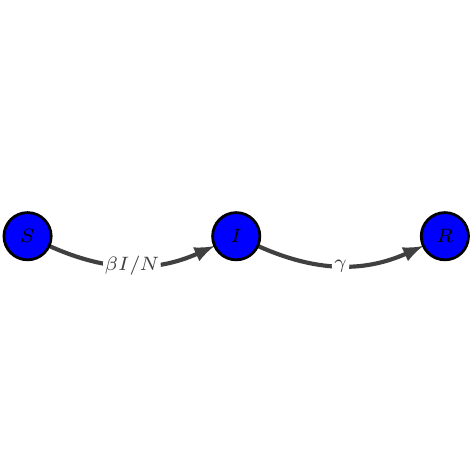
SIR

show_graph(models.sir)

show_latex(models.sir)

$\displaystyle \begin{array}{lcl} \dot{S} &=& -\beta I / N S\\ \dot{I} &=& \beta I / N S - \gamma I\\ \dot{R} &=& \gamma I \end{array}$

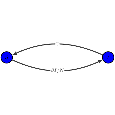
SIS

show_graph(models.sis)

show_latex(models.sis)

$\displaystyle \begin{array}{lcl} \dot{S} &=& -\beta I / N S + \gamma I\\ \dot{I} &=& \beta I / N S - \gamma I \end{array}$

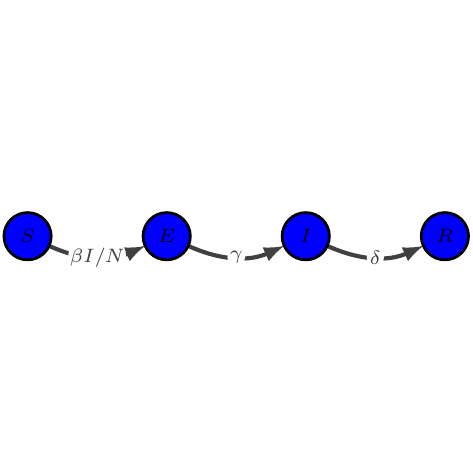
SEIR

show_graph(models.seir)

show_latex(models.seir)

$\displaystyle \begin{array}{lcl} \dot{S} &=& -\beta I / N S\\ \dot{E} &=& \beta I / N S - \gamma E\\ \dot{I} &=& \gamma E - \delta I\\ \dot{R} &=& \delta I \end{array}$

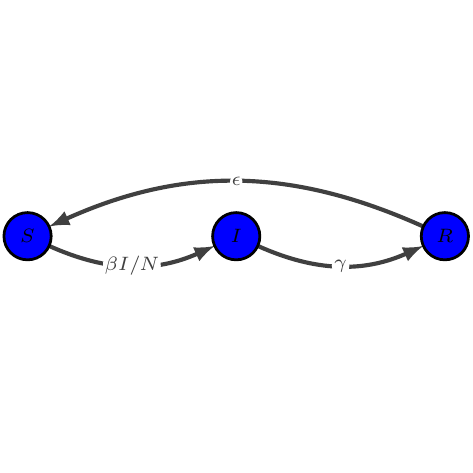
SIRS

show_graph(models.sirs)

show_latex(models.sirs)

$\displaystyle \begin{array}{lcl} \dot{S} &=& -\beta I / N S + \epsilon R\\ \dot{I} &=& \beta I / N S - \gamma I\\ \dot{R} &=& \gamma I - \epsilon R \end{array}$

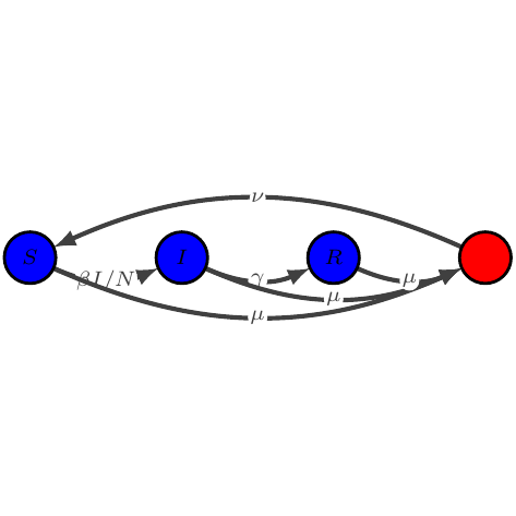
Models with vital dynamics

Models with vital dynamics are easilly created extending an existing model.

from comod import add_natural

show_graph(add_natural(models.sir))

show_latex(add_natural(models.sir))

$\displaystyle \begin{array}{lcl} \dot{S} &=& -\beta I / N S + \nu N - \mu S\\ \dot{I} &=& \beta I / N S - \gamma I - \mu I\\ \dot{R} &=& \gamma I - \mu R \end{array}$