Demo and cookbook

import comod
import numpy as np

Defining a model

Models are defined enumerating the states, parameters and transition rules.

Each of this rules is given by the origin compartment, the destination compartment, and the proportionality coeffient with describes the flow per individual in the origin to the destination.

model = comod.Model(
    ["S", "I", "R"],  # States
    ["beta", "gamma"],  # Coefficients
    [  # Rules in the form (origin, destination, coefficient)
        ("S", "I", "beta I / N"),  # N is a special state with the total population
        ("I", "R", "gamma"),
    ],
    # Special state names can be set with the following options:
    sum_state="N",  # Total population. Can be used in the coefficients, but not as origin/destination.
    nihil_state="!",  # The nothingness (?) from which one is born and to which one dies.
    # Can be used as origin/destination, but not in the cofficients.
)

Plotting the model

Plotting with tikz

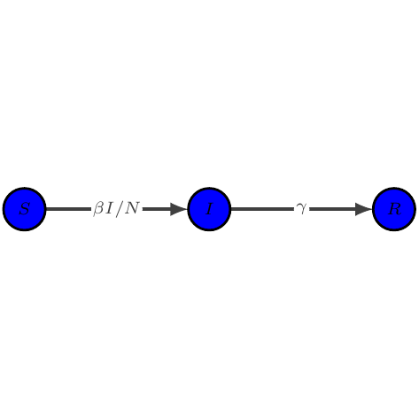
Plotting with tikz might be convenient for the generation of high quaility plots of small models.

model.plot_tikz(layout={"S": (1, 0), "I": (2, 0), "R": (3, 0)})

The generating tex file can be exported for further tweaking.

model.plot_tikz("export_demo.tex", layout={"S": (1, 0), "I": (2, 0), "R": (3, 0)})

!cat export_demo.tex

\documentclass{standalone}
\usepackage{tikz-network}
\begin{document}
\begin{tikzpicture}
\clip (0,0) rectangle (6,6);
\Vertex[x=0.350,y=3.000,color=blue,label=$S$]{S}
\Vertex[x=3.000,y=3.000,color=blue,label=$I$]{I}
\Vertex[x=5.650,y=3.000,color=blue,label=$R$]{R}
\Edge[,label=$\beta I / N$,Direct](S)(I)
\Edge[,label=$\gamma$,Direct](I)(R)
\end{tikzpicture}
\end{document}

Plotting with igraph

Plotting python igraph might be convenient for larger graphs due to its layout capabilities.

model.plot_igraph(layout="circle", bbox=(300, 300 / 1.618))

Output the differential equations in LaTeX

latex = model.to_latex()
print(latex)

\begin{array}{lcl} \dot{S} &=& -\beta I / N S\\
\dot{I} &=& \beta I / N S - \gamma I\\
\dot{R} &=& \gamma I
\end{array}

from IPython.display import display, Math

display(Math(latex))

$\displaystyle \begin{array}{lcl} \dot{S} &=& -\beta I / N S\\ \dot{I} &=& \beta I / N S - \gamma I\\ \dot{R} &=& \gamma I \end{array}$

Solve and plot

Basic solution

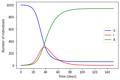
The model can be numerically solved given the values of the parameters and the initial conditions.

t = np.linspace(0, 150, 150)
S, I, R = model.solve(
    (999, 1, 0),  # Initial state
    [0.3, 0.1],  # Coefficient values
    t,  # Time mesh
    method="RK45",  # see scipy.integrate.solve_ivp
)

import matplotlib.pyplot as plt

plt.plot(t, S, "b", label="S")
plt.plot(t, I, "r", label="I")
plt.plot(t, R, "g", label="R")
plt.xlabel("Time [days]")
plt.ylabel("Number of individuals")
plt.legend()
plt.show()

Dynamic solution using ipywidgets

Interactive visualization using ipywidgets. Only available when running as a notebook.

import ipywidgets

@ipywidgets.interact
def plot(
    beta=ipywidgets.FloatSlider(min=0.0, max=2, value=0.3, description="$\\beta$"),
    gamma=ipywidgets.FloatSlider(
        min=0.0, max=0.3, value=0.1, step=0.01, description="$\\gamma$"
    ),
):
    t = np.linspace(0, 150, 150)
    S, I, R = model.solve((999, 1, 0), [beta, gamma], t)
    plt.plot(t, S, "b", label="S")
    plt.plot(t, I, "r", label="I")
    plt.plot(t, R, "g", label="R")
    plt.xlabel("Time [days]")
    plt.ylabel("Number of individuals")
    plt.legend()
    plt.show()

Time-dependent parameter solution

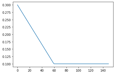
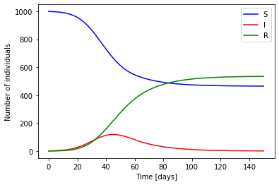
The model can also be solved if the parameters are functions of time

def beta_time(t):
    return max(0.1, 0.3 - t / 30 * 0.1)

plt.plot([beta_time(x) for x in t])
plt.show()

solution_time = model.solve_time(
    (999, 1, 0),  # Initial state
    [beta_time, lambda x: 0.1],  # Coefficient values
    t,  # Time mesh
)

import matplotlib.pyplot as plt

plt.plot(t, solution_time[0], "b", label="S")
plt.plot(t, solution_time[1], "r", label="I")
plt.plot(t, solution_time[2], "g", label="R")
plt.xlabel("Time [days]")
plt.ylabel("Number of individuals")
plt.legend()
plt.show()

Best fit

Use the previously generated data to best-fit a model.

fit_pars = model.best_fit(
    np.asarray([S, I, R]), t, [0.2, 0.2]  # Existing data  # Time mesh  # Initial guess
).x

print("Fitted parameters:")
for par, value in zip(model.parameters, fit_pars):
    print("%s: %.3f" % (par, value))

Fitted parameters:
beta: 0.298
gamma: 0.101

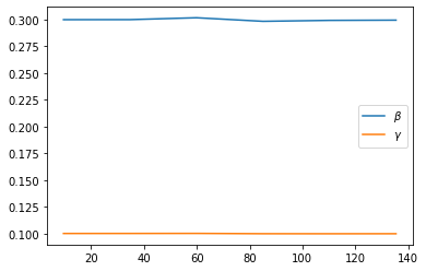
Best fit in time windows

Fits can be performed using sliding windows.

First, let’s try with the constant model:

results = model.best_sliding_fit(
    np.asarray([S, I, R]),  # Existing data
    t,  # Time mesh
    [0.2, 0.2],  # Initial guess
    window_size=20,  # Window size
    step_size=25,  # Number of time steps between windows
    target="y",  # The target to minimize can be "y" (values) or "dy" (their derivatives)
)
results

	beta	gamma
9.563758	0.300000	0.100001
34.731544	0.300037	0.100028
59.899329	0.301793	0.100076
85.067114	0.298463	0.099781
110.234899	0.299341	0.099746
135.402685	0.299556	0.099773

plt.plot(results)
plt.legend(["$\\beta$", "$\\gamma$"])
plt.show()

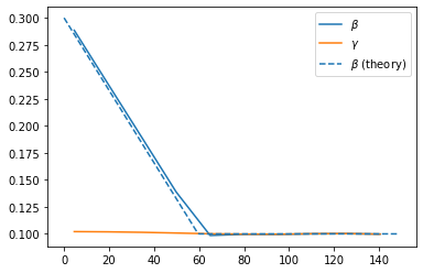
Now let’s try the time-dependent coefficient model

results = model.best_sliding_fit(
    solution_time,  # Existing data
    t,  # Time mesh
    [0.2, 0.2],  # Initial guess
    window_size=10,  # Window size
    step_size=15,  # Number of time steps between windows
    target="y",  # The target to minimize can be "y" (values) or "dy" (their derivatives)
    time_criterion="mean",  # Determines how a time is assigned to each window in the solution
)
results

	beta	gamma
4.530201	0.288520	0.102111
19.630872	0.238503	0.101901
34.731544	0.188711	0.101453
49.832215	0.138761	0.100800
64.932886	0.098525	0.100100
80.033557	0.099614	0.099815
95.134228	0.099563	0.099749
110.234899	0.100074	0.100113
125.335570	0.100256	0.100254
140.436242	0.099812	0.099812

plt.plot(results)
plt.plot([beta_time(x) for x in t], "C0--")
plt.legend(["$\\beta$", "$\\gamma$", "$\\beta$ (theory)"])
plt.show()

Symbolic calculation of fixed points

A sympy represenation of the model can automatically be obtained if the package is installed:

model.get_sympy()

$\displaystyle \left[\begin{matrix}- \frac{1.0 I S \beta}{I + R + S}\\\frac{1.0 I S \beta}{I + R + S} - 1.0 I \gamma\\1.0 I \gamma\end{matrix}\right]$

An automatic calculation of fixed points can be performed for simple models.

for point, jacobian in model.get_fixed_points():
    print("Fixed point:")
    display(point)
    print("Jacobian:")
    display(jacobian)

Fixed point:

(S, 0.0, R)

Jacobian:

$\displaystyle \left[\begin{matrix}0 & - \frac{1.0 S \beta}{R + S} & 0\\0 & \frac{1.0 S \beta}{R + S} - 1.0 \gamma & 0\\0 & 1.0 \gamma & 0\end{matrix}\right]$

jacobian.eigenvals()

{-(R*gamma - S*beta + S*gamma)/(R + S): 1, 0: 2}

Stability analysis is left as an exercise for the reader.